Count real roots by isolating a parameter: a graphical method

The idea: keep the curve fixed and move a line

Suppose you need to count the real solutions of an equation containing a real parameter $a$. Rather than tracking a different complicated graph for every $a$, rearrange the equation so that one graph is fixed and the other is simple.

For example,

$$x^2-ax+1=0\quad\Longleftrightarrow\quad x^2+1=ax.$$

A root is the $x$-coordinate of an intersection between the fixed parabola $y=x^2+1$ and the line $y=ax$. Changing $a$ rotates the line about the origin. In Japanese entrance-exam mathematics this rearrangement is often called parameter separation.

This is a graphical counting technique, not separation of variables for differential equations. Its purpose is to make the changing part of the problem easy to understand.

A four-step method

1. Separate the parameter-dependent terms from the remaining terms.
2. Draw the two graphs, including all domain restrictions.
3. Find parameter values where they touch, cross an endpoint, or encounter a discontinuity.
4. Count intersections between and at those critical values.

The fourth step matters: finding a tangent does not by itself establish how many roots exist elsewhere.

Worked example: exactly one root in an open interval

Problem. Find all real $a$ for which

$$x^2+2ax-a+1=0$$

has exactly one distinct real root in $-1<x<3$. A double root counts as one distinct root.

Step 1: separate the parameter

Rearrange as

$$-x^2-1=2ax-a=2a\left(x-\frac12\right).$$

Compare the fixed curve $y=-x^2-1$ with a line passing through $(1/2,0)$. Only the line's slope changes.

Step 2: find the tangencies

A tangency corresponds to a double root. The discriminant of the original quadratic is

$$D=4(a^2+a-1).$$

Thus tangency occurs at

$$a=\frac{-1-\sqrt5}{2}\quad\text{or}\quad a=\frac{-1+\sqrt5}{2}.$$

The double root is $x=-a$. For both values, it lies inside $(-1,3)$, so both tangencies contribute a valid answer.

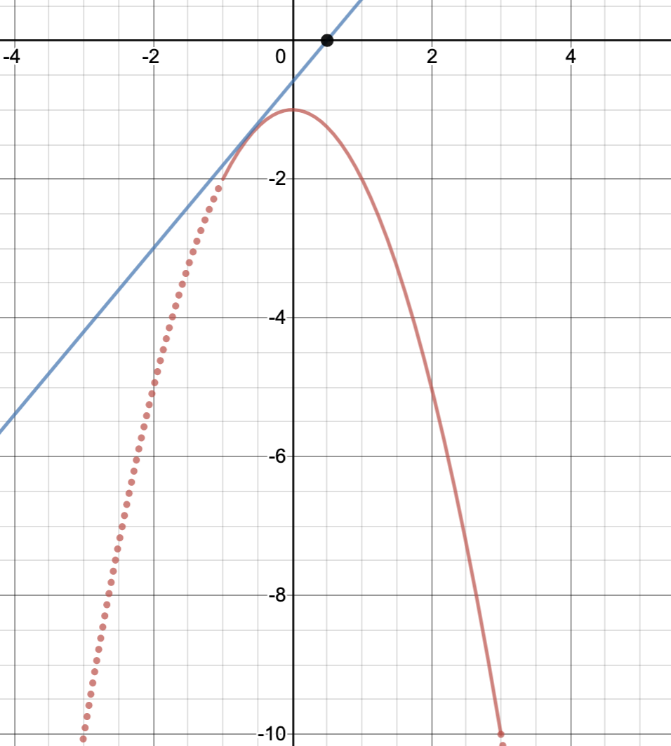
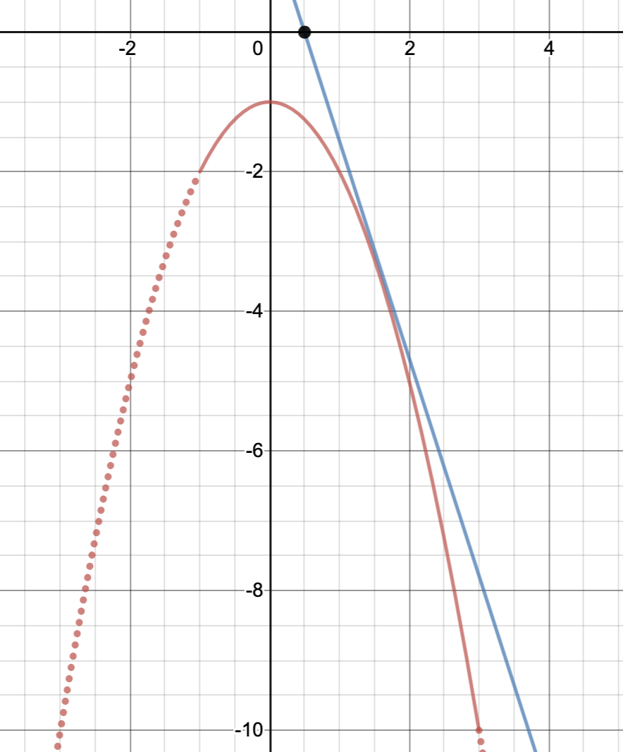
Step 3: find the endpoint crossings

Substitute the endpoints into the original polynomial $F_a(x)=x^2+2ax-a+1$:

$$F_a(-1)=2-3a,\qquad F_a(3)=10+5a.$$

The crossing values are $a=2/3$ and $a=-2$, respectively. Notice that $F_a(-1)=0$ means $a=2/3$: the fixed graph has height $-2$ at $x=-1$, not $2$.

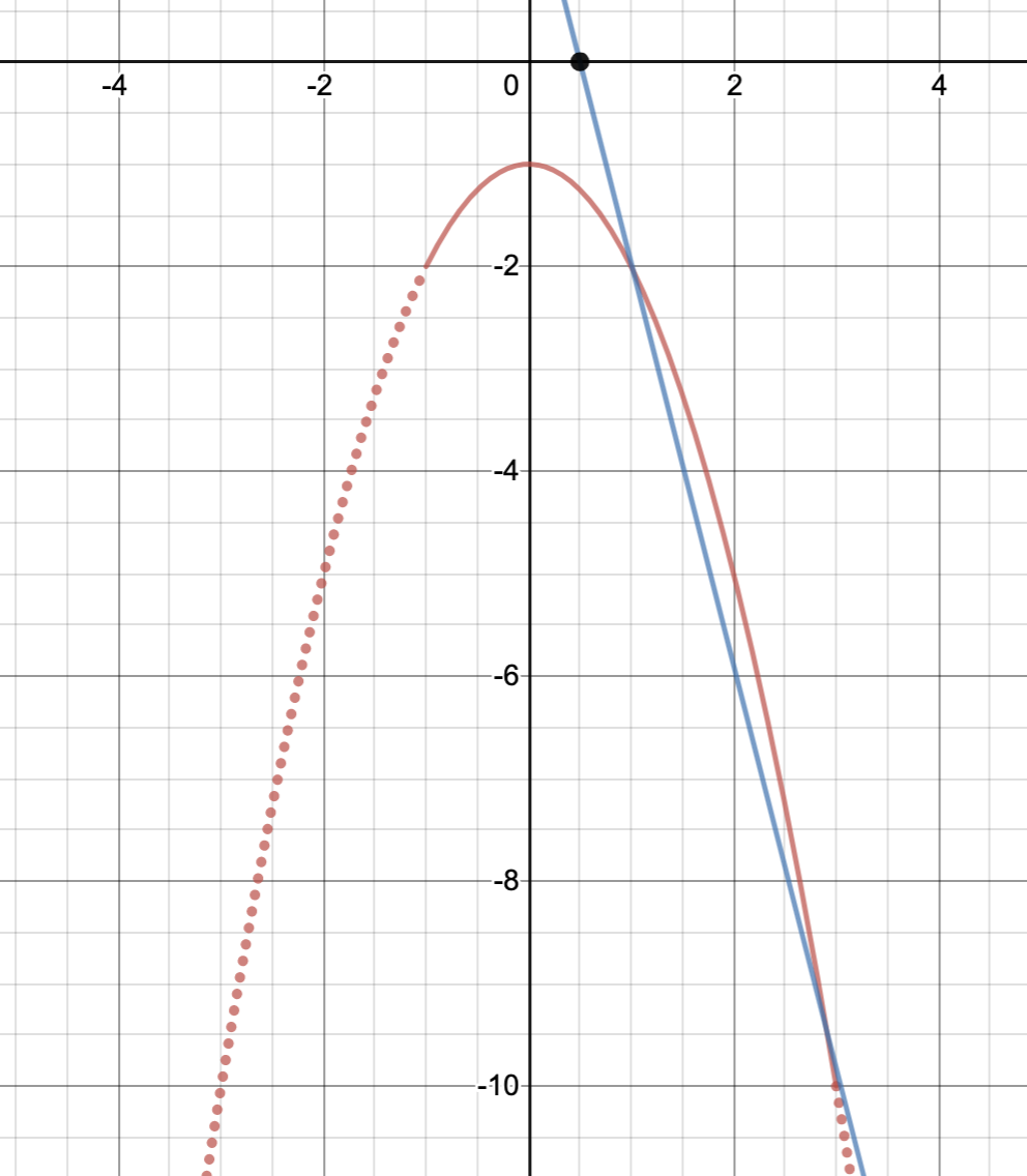
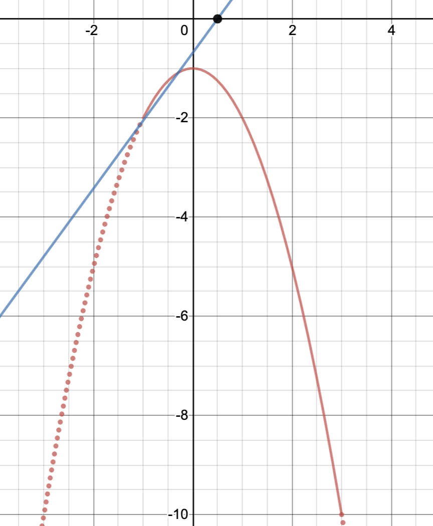
Step 4: count roots, including the critical cases

Let $a_-=(-1-\sqrt5)/2$ and $a_+=(-1+\sqrt5)/2$. The four critical values are ordered as

$$-2<a_-<a_+<\frac23.$$

• If $a<-2$, the two endpoint values have opposite signs, so exactly one root lies in the interval.
• At $a=-2$, the roots are $1$ and $3$. Only $1$ lies in the open interval.
• If $-2<a<a_-$, there are two distinct roots inside the interval.
• At $a=a_-$, there is one double root inside.
• If $a_-<a<a_+$, the discriminant is negative, so there are no real roots.
• At $a=a_+$, there is one double root inside.
• If $a_+<a<2/3$, there are two distinct roots inside.
• At $a=2/3$, the roots are $-1$ and $-1/3$. Only $-1/3$ lies inside.
• If $a>2/3$, the endpoint values again have opposite signs, giving exactly one root inside.

Therefore the answer is

$$\boxed{a\le-2\quad\text{or}\quad a=\frac{-1\pm\sqrt5}{2}\quad\text{or}\quad a\ge\frac23.}$$

The endpoint values are included in the answer even though the interval is open: in each case, one root is excluded at an endpoint while the other remains inside.

When is this method useful?

The rearrangement is especially convenient when the parameter-dependent graph becomes a horizontal line or a line through a fixed point. It is often more revealing for square roots, absolute values, reciprocal functions, or step functions than repeatedly solving algebraic equations.

These are favorable situations, not necessary conditions. A parameter need not appear only to the first power, and the moving graph need not always be a line. For instance, $x^2=a^2$ can still be analyzed using a horizontal line of height $a^2$. The question is whether the rearrangement makes the geometry easier.

For an ordinary quadratic, the discriminant, vertex, and endpoint signs may be quicker. Use the graph when it clarifies the structure, rather than forcing every problem into this method.

Application 1: a square-root curve

Problem. Count the real solutions of

$$\sqrt{x-1}=ax.$$

Domain and sign first

The domain is $x\ge1$. Since $x>0$ and the square root is nonnegative, there are no solutions for $a<0$. If $a=0$, the unique solution is $x=1$.

For $a>0$, compare $y=\sqrt{x-1}$ with $y=ax$.

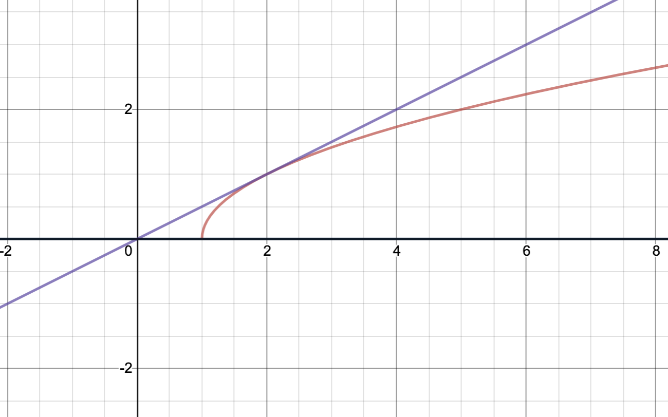
Squaring is reversible only when the signs are correct:

$$\sqrt{x-1}=ax\quad\Longleftrightarrow\quad a^2x^2-x+1=0,\quad x\ge1,\quad ax\ge0.$$

The discriminant is $1-4a^2$, so the positive tangent value is $a=1/2$, with $x=2$.

To verify the root count without relying on a sketch, solve for the parameter:

$$a=h(x)=\frac{\sqrt{x-1}}x,\qquad x\ge1.$$

This function rises from $0$ to $1/2$ at $x=2$, then decreases toward $0$ without reaching it again. Consequently:

• $a<0$: no roots.
• $a=0$: one root, $x=1$.
• $0<a<1/2$: two distinct roots.
• $a=1/2$: one root, $x=2$.
• $a>1/2$: no roots.

Squaring first and forgetting the sign condition would incorrectly suggest solutions for negative $a$.

Application 2: a semicircle and a rotating line

Problem. Count the real solutions of

$$\sqrt{1-x^2}-ax-2a=0.$$

The domain is $-1\le x\le1$, and separation gives

$$\sqrt{1-x^2}=a(x+2).$$

The fixed curve is the upper unit semicircle. The line passes through $(-2,0)$, so its slope determines how it crosses the semicircle.

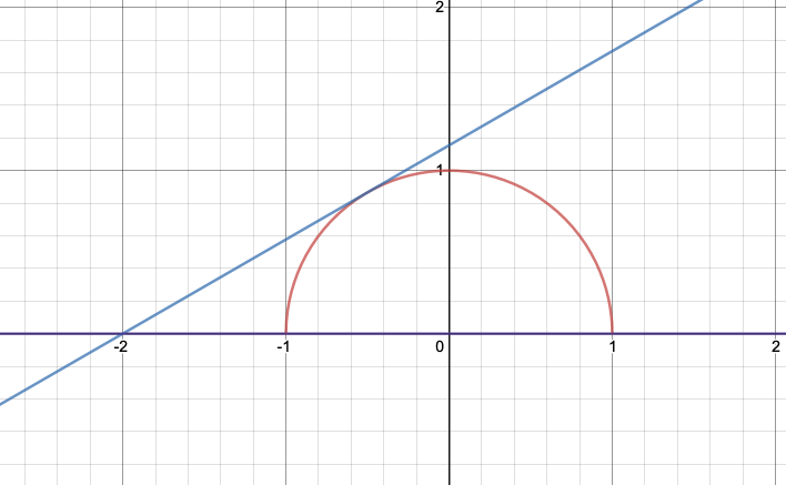
Because $x+2>0$ on the entire domain, negative $a$ gives no roots. At $a=0$, both endpoints $x=-1,1$ are roots.

For positive $a$, tangency occurs when the distance from the origin to the line $ax-y+2a=0$ equals the unit radius:

$$\frac{2a}{\sqrt{a^2+1}}=1\quad\Longleftrightarrow\quad a=\frac1{\sqrt3}.$$

At this value, the contact point has $x=-1/2$ and lies on the upper semicircle. Therefore:

• $a<0$: no roots.
• $0\le a<1/\sqrt3$: two distinct roots.
• $a=1/\sqrt3$: one root, $x=-1/2$.
• $a>1/\sqrt3$: no roots.

The negative-slope tangent to the full circle does not touch the upper semicircle. Working with the correct half of the circle prevents an extra, invalid critical value.

Application 3: the floor function and half-open endpoints

Problem. Let $\lfloor x\rfloor$ denote the greatest integer not exceeding $x$. Count the distinct real solutions of

$$\lfloor x\rfloor=ax,\qquad 2\le x<4.$$

On this domain,

$$\lfloor x\rfloor=\begin{cases}2,&2\le x<3,\\3,&3\le x<4.\end{cases}$$

The graph consists of two horizontal segments, each closed on the left and open on the right.

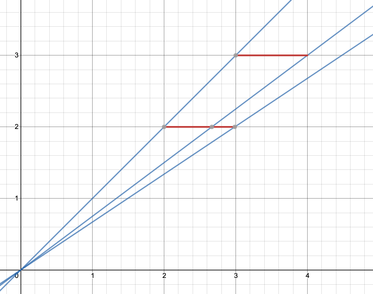
For the first segment, a solution must be $x=2/a$. Its interval restriction gives

$$2\le\frac2a<3\quad\Longleftrightarrow\quad\frac23<a\le1.$$

For the second, a solution must be $x=3/a$, and

$$3\le\frac3a<4\quad\Longleftrightarrow\quad\frac34<a\le1.$$

There are no solutions when $a\le0$. Combining the two positive-parameter ranges:

• $a\le2/3$: no roots.
• $2/3<a\le3/4$: one root.
• $3/4<a\le1$: two distinct roots.
• $a>1$: no roots.

At $a=3/4$, the candidate $x=4$ is excluded, so only the first segment contributes. At $a=1$, both left endpoints, $x=2$ and $x=3$, are included.

A final checklist

Identify the domain before manipulating the equation. Track signs before squaring. Check tangencies, endpoints, and discontinuities separately. Finally, explain why the roots of the original equation correspond exactly to the intersections you counted.

This same change of viewpoint also helps with regions swept out by a moving line. For another example of domain checks in a geometric problem, see circle inversion.