Factoring 21 with Shor's algorithm: qubits, periods, and retries

The quantum part finds an order

Shor's factoring algorithm combines a quantum order-finding subroutine with classical arithmetic. For coprime positive integers $a,N$, the multiplicative order of $a$ modulo $N$ is the least positive integer $r$ satisfying

$$a^r\equiv1\pmod N.$$

Our target is $N=21$. We first use $a=5$, as in the original article, and discover why even a correctly found order can fail to give a factor. We then use $a=2$ to finish the factorization.

The small circuit below is an illustration of interference, not a register-size prescription for reliable large-number factoring. The full algorithm and its efficiency analysis are given in Peter Shor's original paper.

1. Qubits and measurement

A pure qubit state is

$$\alpha|0\rangle+\beta|1\rangle, \qquad\alpha,\beta\in\mathbb C,\quad|\alpha|^2+|\beta|^2=1.$$

Measurement in this computational basis returns zero with probability $|\alpha|^2$ and one with probability $|\beta|^2$. The coefficients are amplitudes, not probabilities themselves. A global complex phase does not change the physical pure state; the Bloch sphere describes pure states after this equivalence, rather than arbitrary real unit vectors representing all register states.

Independent registers combine by tensor product. For example,

$$\begin{aligned} &\frac{|0\rangle+|1\rangle}{\sqrt2} \otimes\left(\frac12|0\rangle+\frac{\sqrt3i}{2}|1\rangle\right)\\ &=\frac1{2\sqrt2}|00\rangle+\frac{\sqrt3i}{2\sqrt2}|01\rangle +\frac1{2\sqrt2}|10\rangle+\frac{\sqrt3i}{2\sqrt2}|11\rangle. \end{aligned}$$

The four outcome probabilities are $1/8,3/8,1/8,3/8$, summing to one. This particular state is a product state, not an entangled state. A general multi-qubit state need not factor into a product of individual qubits.

We abbreviate tensor products of basis states using binary strings, or their decimal values when the register width is understood. Thus $|1101\rangle=|13\rangle$ in a four-qubit register. The symbol $|1\rangle$ can describe a single qubit or a multi-qubit register encoding the integer one, so the register size must be stated.

2. Hadamard gates and controlled operations

The Hadamard gate acts as

$$H|0\rangle=\frac{|0\rangle+|1\rangle}{\sqrt2},\qquad H|1\rangle=\frac{|0\rangle-|1\rangle}{\sqrt2}.$$

Applying it to each qubit of an initially zero $n$-qubit register creates

$$H^{\otimes n}|0\cdots0\rangle =\frac1{\sqrt{2^n}}\sum_{x=0}^{2^n-1}|x\rangle.$$

A controlled operation applies $U$ when the control is one and the identity when it is zero. It acts linearly on a superposition, and can create entanglement. A controlled bit flip, for example, maps

$$\frac{|0\rangle+|1\rangle}{\sqrt2}\otimes|0\rangle \longmapsto\frac{|00\rangle+|11\rangle}{\sqrt2}.$$

Hadamards alone do not implement Shor's algorithm: reversible modular arithmetic, controlled operations, and phase operations for the Fourier transform are also needed.

3. The quantum Fourier transform

On a register with $Q=2^n$ basis states, use the convention

$$F_Q|j\rangle=\frac1{\sqrt Q}\sum_{m=0}^{Q-1}e^{2\pi imj/Q}|m\rangle,$$ $$F_Q^{-1}|j\rangle=\frac1{\sqrt Q}\sum_{m=0}^{Q-1}e^{-2\pi imj/Q}|m\rangle.$$

These are unitary transformations. Their phases make some contributions reinforce and others cancel. Order finding uses this interference to obtain information about a period; it does not read out all values calculated in a superposition.

4. Prepare a small order-finding example

Take four control qubits, so $Q=16$, and a five-qubit work register initialized to the integer one. Five qubits are needed for general residues modulo 21, including the value 20. Four work qubits would not suffice; the original text's register counts are inconsistent.

For $0\le y<21$, define

$$U|y\rangle=|5y\bmod21\rangle.$$

Because five is coprime to 21, this is a permutation of those 21 basis states. Define $U$ to fix the remaining basis states $21,\ldots,31$ to obtain a unitary permutation on the entire five-qubit register.

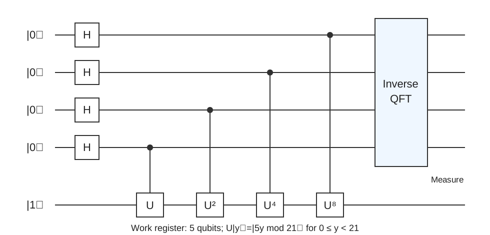
Write $x=x_0+2x_1+4x_2+8x_3$. The control bit $x_k$ applies $U^{2^k}$, so their product applies $U^x$ and maps the work state one to $5^x\bmod21$. The powers are implemented by modular repeated-squaring circuits, not by literally repeating an enormous number of gates.

After the Hadamards and controlled modular operations, the joint state is

$$|\Psi\rangle=\frac14\sum_{x=0}^{15}|x\rangle|5^x\bmod21\rangle.$$

The residues repeat with period six:

| $x\bmod6$ | $5^x\bmod21$ | Control values in this example | | --- | --- | --- | | 0 | 1 | 0, 6, 12 | | 1 | 5 | 1, 7, 13 | | 2 | 4 | 2, 8, 14 | | 3 | 20 | 3, 9, 15 | | 4 | 16 | 4, 10 | | 5 | 17 | 5, 11 |

Thus the grouped state is

$$\begin{aligned} |\Psi\rangle=\frac14\big[&(|0\rangle+|6\rangle+|12\rangle)|1\rangle +(|1\rangle+|7\rangle+|13\rangle)|5\rangle\\ &+(|2\rangle+|8\rangle+|14\rangle)|4\rangle +(|3\rangle+|9\rangle+|15\rangle)|20\rangle\\ &+(|4\rangle+|10\rangle)|16\rangle +(|5\rangle+|11\rangle)|17\rangle\big]. \end{aligned}$$

The second ket in each product is a five-qubit register. There are sixteen orthogonal joint terms, each with amplitude $1/4$, so the state is normalized.

We can see the period in a written table, but measuring the state does not return that table: it returns one basis outcome. The algorithm must convert the periodic structure into measurable interference.

5. Fourier interference reveals the period structure

For explanation, imagine measuring the work register. If the result is one, which occurs with probability $3/16$, the normalized control state becomes

$$\frac{|0\rangle+|6\rangle+|12\rangle}{\sqrt3}.$$

After the inverse QFT, its amplitude at outcome $m$ is

$$A_m=\frac1{4\sqrt3}\left(1+e^{-2\pi im6/16}+e^{-2\pi im12/16}\right).$$

Consequently,

$$\Pr(m\mid\text{work}=1)=\frac1{48} \left|1+e^{-2\pi im6/16}+e^{-2\pi im12/16}\right|^2.$$

This compact normalized expression avoids the missing factors and incorrect expanded coefficients in the source.

More generally, a work outcome selects control values $b,b+r,\ldots,b+(L-1)r$, all below $Q$. Their normalized post-measurement state transforms to amplitudes

$$A_m=\frac{e^{-2\pi imb/Q}}{\sqrt{QL}} \sum_{\ell=0}^{L-1}e^{-2\pi imr\ell/Q}.$$

The prefactor has unit-magnitude phase apart from normalization. The finite geometric sum is large when neighboring phases are nearly aligned:

$$\frac{mr}{Q}\approx k, \qquad\text{or}\qquad\frac mQ\approx\frac kr.$$

When the denominator below is nonzero, the squared magnitude of that sum is

$$\frac{\sin^2(\pi Lmr/Q)}{\sin^2(\pi mr/Q)}.$$

At exact alignment its limiting value is $L^2$. This explains the peaks rather than asserting that the Fourier transform deterministically outputs the period.

The work measurement is optional. Measuring only the transformed control register gives the mixture over the work outcomes. For $Q=16$ and $r=6$, the exact marginal probabilities are approximately:

| Outcomes $m$ | Probability of each listed outcome | | --- | --- | | 0, 8 | 0.17187500 | | 3, 5, 11, 13 | 0.11774272 | | 2, 6, 10, 14 | 0.03125000 | | 4, 12 | 0.01562500 | | 1, 7, 9, 15 | 0.00725728 |

They sum to one. The largest peaks lie near multiples of $Q/r=16/6$, namely $0,3,5,8,11,13$. Other outcomes remain possible, and different conditioned work outcomes need not have identical finite-register distributions.

6. Recovering and checking a candidate order

A measured $m$ suggests a rational approximation $m/Q\approx k/r$. A reduced fraction may reveal only a divisor of $r$ when $k$ and $r$ share a factor. The outcome $m=0$ is also uninformative about the order by itself.

For the standard precision argument, choose a sufficiently large power-of-two control range, conventionally $N^2\le Q<2N^2$. Continued fractions recover candidate denominators from good approximations; candidates must be checked by modular exponentiation, and repetitions or suitable multiples may be needed. The four-control-qubit example has $Q=16<21^2$, so recognizing its histogram is not a general guarantee of successful continued-fraction recovery. The precision and postprocessing argument is developed in Shor's order-finding analysis, Section 5.

In this small example, direct arithmetic checks the candidate six:

$$5^1,5^2,\ldots,5^6\pmod{21}=5,4,20,16,17,1.$$

No earlier power is one, so the order is exactly six. For large inputs, the point of the quantum subroutine is to avoid a linear search through all these powers.

7. Why base five fails to factor 21

Before order finding, compute $\gcd(a,N)$. A nontrivial gcd already gives a factor; otherwise proceed with a coprime base. If its order $r$ is odd, the usual factoring step cannot use $a^{r/2}$, so choose another base.

For even $r$,

$$a^r-1=(a^{r/2}-1)(a^{r/2}+1)\equiv0\pmod N.$$

Compute the two gcds with $N$. A nontrivial result between one and $N$ is a factor, though not necessarily a prime factor for a general composite input.

For $a=5$, $r=6$,

$$5^3=125\equiv-1\pmod{21},$$

so

$$\gcd(124,21)=1,\qquad\gcd(126,21)=21.$$

Neither is a nontrivial factor. An even order alone is insufficient: this base's half-order power is minus one modulo the whole input.

8. Retry with base two and finish

For $a=2$, the order is also six:

$$2^1,2^2,\ldots,2^6\pmod{21}=2,4,8,16,11,1.$$

Now $2^3=8$ is neither one nor minus one modulo 21. The gcds are

$$\gcd(2^3-1,21)=\gcd(7,21)=7,$$ $$\gcd(2^3+1,21)=\gcd(9,21)=3.$$

Therefore

$$\boxed{21=3\cdot7.}$$

The workflow is: choose a base, check its gcd, find and verify an order, try the half-order gcds, and retry when they are unhelpful. The quantum component supplies information about a period through interference; the final factor extraction is ordinary integer arithmetic.